What has to be true before a GPON estate can carry XGS-PON?
A GPON to XGS-PON upgrade is not an OLT swap. The headend is the easy half: a board goes in, a coexistence element goes in front of it, a new port appears. The hard half is the passive plant built for 2.5 Gbps, now expected to carry 1577 nm light at 10 Gbps to the same ONU positions.
That difference shows up as arithmetic. A GPON port at 2.5 Gbps shared by 32 subscribers averages about 78 Mbps each if everyone downloads at once, which is why a mature estate needs 10G for headroom rather than for a single subscriber speed. XGS-PON answers with 10 Gbps each way and reuses the ODN instead of the trench, so the ODN is what has to be proven first.
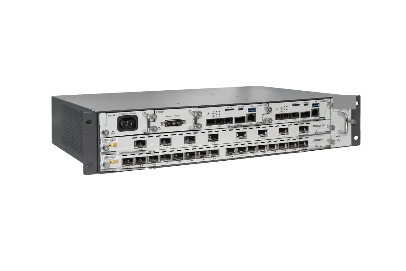
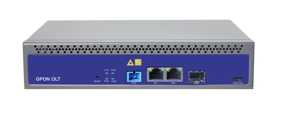
Three conditions decide whether the reuse is honest: the measured end-to-end loss per PON port must sit inside the XGS-PON optical class with reserve left for ageing; every GPON ONU staying on the shared fibre must accept the reduced upstream band; and the splitters and connectors must be rated across 1260–1650 nm. The 10G PON OLT page lists the chassis options; this note is the sequence that decides how many boards the plant can support.
Which ODN measurements decide the migration?
Measure at 1577 nm and 1270 nm where the instrument allows, and record the wavelength with every reading. A clean 1310 nm number says almost nothing about the 1577 nm loss in the same link, because attenuation, macrobend loss and connector behaviour all differ across the band.
Start from the records that already exist: as-built route length, splitter ratios, the per-port test data supplied with the hardware, splice count per span and connector polish at every termination. Then verify the record on site. Per-port splitter data is the fastest check, because an output that has drifted 2 dB from its factory figure explains a marginal subscriber better than any OTDR trace. Where no factory data exists, measure through-loss output by output on a dark port and write the value on the closure label.
The audit ends with one number per PON port: worst-case loss from OLT connector to ONU connector at the wavelength that matters. That number, not the split ratio on the drawing, is compared with the optical class. The optical link budget guide sets out the form; the field rule is to fill it with measured values and mark every assumed value as assumed.
| Audit item | How it is measured | Pass criterion |
|---|---|---|
| End-to-end loss per PON port | Light source and power meter, or OTDR on a dark port | Inside the class, with reserve |
| Splitter per-port loss | Factory data, verified by spot measurement | Within datasheet tolerance |
| Splitter band | Datasheet model number | Rated 1260–1650 nm |
| Connector polish | Visual and mechanical check | APC to APC, UPC to UPC |
| Splice count per span | Closure inspection | Matches the as-built |
| GPON ONU inventory | Model, firmware, wavelength range | Supports the reduced band |
| Reserve fibre | Count at each closure | Enough for the new service |
The audit is a record, not a survey: estimated values are marked and re-measured before cutover.
Why do wavelengths decide whether the ODN can be shared?
GPON transmits at 1490 nm downstream and 1310 nm upstream; XGS-PON transmits at 1577 nm and 1270 nm. Downstream, the bands are far apart and a filter separates them cleanly. Upstream they are not: the XGS-PON band at 1260–1280 nm sits inside the lower edge of the wide GPON range.
The two generations only share a fibre upstream when the GPON ONUs on it use the reduced upstream range of 1290–1330 nm. That one sentence is the most expensive line in the project: an estate of ONUs that guarantee only the regular band cannot be overlaid as it stands. The inventory becomes a commercial document, because it sets the replacement count and the field visits.
Downstream mirrors the problem. XGS-PON ONUs filter 1490 nm internally; older GPON ONUs may not block 1577 nm, and the strong 10G light then desensitises the 2.5G receiver, which appears as intermittent loss rather than a clean failure. A blocking filter fixes it, at the cost of a connector pair and about 0.5 dB of budget.
| Link | GPON | XGS-PON | Coexistence rule |
|---|---|---|---|
| Downstream | 1480–1500 nm | 1575–1581 nm | Filter separates the bands |
| Upstream, regular | 1260–1360 nm | 1260–1280 nm | Overlap: no coexistence |
| Upstream, reduced | 1290–1330 nm | 1260–1280 nm | Separated: the coexistence condition |
| Line rate | 2.5 / 1.25 Gbps | 10 / 10 Gbps | Does not change the loss budget |
| Fibre | G.652D / G.657A2 | G.652D / G.657A2 | Same fibre; parts must cover the band |
Ranges follow the ITU-T GPON and XGS-PON specifications. Confirm reduced-band support on the ONU datasheet, not on the order description.
Combo port or external coexistence element?
There are two accepted ways to put both generations on one fibre. A combo line card integrates the multiplexing on the card, so one port serves both and the rack stays small. An external coexistence element sits in front of the existing OLT ports, which suits an estate that keeps its GPON chassis and adds 10G boards beside it.
The choice follows what happens next. A combo card locks both services to the same card. An external element is passive, can carry an RF video overlay or an out-of-band OTDR wavelength, and can be swapped for a wider-band unit when a third generation arrives. The trade is rack space, one more patch field and one more loss line.
Either way, the element sits in the light path, so its insertion loss belongs in the budget: typically 0.6–1.2 dB depending on how many services the module integrates. Band isolation matters as much, because downstream light leaking into the upstream burst receiver produces sync errors that look like a dirty connector. Ask for both figures on the datasheet. Where a chassis, its boards and a coexistence element are quoted together, they are specified as one chain with the splitter and patch cords; the 10G PON ONU page covers the subscriber end.
| Criterion | Combo line card | External element |
|---|---|---|
| Rack space | One card, no shelf | One shelf plus patch field |
| Existing GPON chassis | Needs a chassis offering the card | Works ahead of current ports |
| Insertion loss | Lower, internal | 0.6–1.2 dB to budget |
| RF or OTDR overlay | Limited by the card | Supported by module choice |
| Change one generation | Card change | Passive module change |
| Failure mode | Both services on the card | Shared feeder only |
Loss and isolation are module-specific. Confirm them before the split ratio is frozen.
How does coexistence loss change the split ratio?
Run the budget in one direction, from OLT connector to ONU connector, with every line visible. Take a 20 km span on G.652D fibre at 0.25 dB/km for 1577 nm, two connector pairs at 0.5 dB, eight splices at 0.1 dB, and a coexistence element at 1.2 dB.
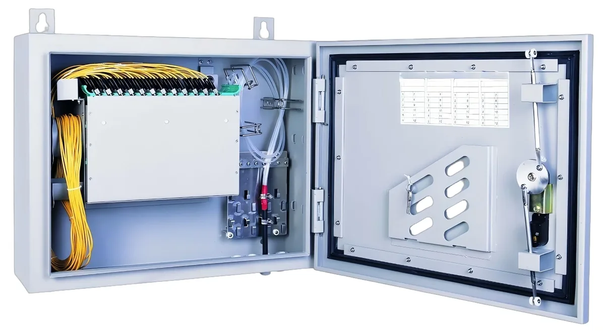
Add the splitter: 16.5 dB for 1:32 and 20.5 dB for 1:64 are the figures published for the fibre splitter family. Against class N1 at 29 dB, the 1:32 case totals 24.5 dB and leaves 4.5 dB; the 1:64 case totals 28.5 dB and leaves 0.5 dB. A half-decibel margin is not a design, and a 3 dB reserve for ageing and repairs turns it negative.
Coexistence is therefore not loss-free, and the consequence is a split ratio decision: reduce to 1:32 on long spans, move the split point deeper so the feeder stays short, or specify optics that meet class N2 at 31 dB. Fix the number before the splitter order, because a 1:64 that has to be replaced after the audit is the most expensive mistake here. The loss table sits in the splitter ratio guide.
| Span | Split | Splitter | Fibre | Connectors and splices | Coexistence | Total | Margin vs N1 | After 3 dB reserve |
|---|---|---|---|---|---|---|---|---|
| 10 km | 1:32 | 16.5 dB | 2.5 dB | 1.8 dB | 1.2 dB | 22.0 dB | 7.0 dB | 4.0 dB |
| 10 km | 1:64 | 20.5 dB | 2.5 dB | 1.8 dB | 1.2 dB | 26.0 dB | 3.0 dB | 0.0 dB |
| 20 km | 1:32 | 16.5 dB | 5.0 dB | 1.8 dB | 1.2 dB | 24.5 dB | 4.5 dB | 1.5 dB |
| 20 km | 1:64 | 20.5 dB | 5.0 dB | 1.8 dB | 1.2 dB | 28.5 dB | 0.5 dB | -2.5 dB |
Class N1 is 29 dB per ITU-T G.9807.1. Substitute the measured audit values and the datasheet figures before committing the ratio.
What does the cutover sequence look like on site?
Migrate by cluster, not by estate. A cluster is one splitter group or one building riser: the largest unit that can be cut over, measured and rolled back inside a maintenance window. Prove the headend, light one pilot port with a known-good ONU, migrate a pilot cluster, measure the post-cutover power at every ONU in it, then batch the rest.
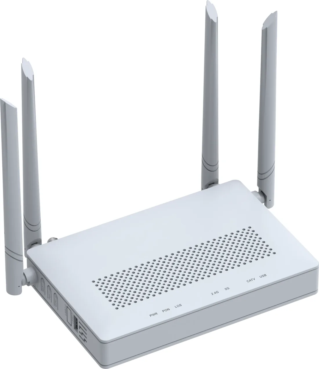
Keep the two services separate above the physical layer: the 10G service gets its own VLAN, QoS profile and provisioning template, because the two generations share light, not configuration. On the subscriber side the LAN port spoils the upgrade most often, since a 10 Gbps PON port feeding a 1GE ONU delivers a 1GE service until the ONU exposes a 10GE or 2.5GE port.
Downtime per subscriber is minutes. The real cost is the truck-roll count, driven by how many ONUs are replaced rather than re-provisioned, and that count comes straight out of the audit.
- Audit and freeze the per-port loss figures before the board order.
- Install the coexistence element and 10G boards; leave the GPON path untouched.
- Light one pilot port and register a known-good ONU before subscriber work.
- Migrate one cluster, measure every ONU, record the value.
- Keep the old profile and old ONU until the cluster has passed.
- Retire the GPON board only when the port has no GPON ONUs left.
Where does the migration money go?
Industry estimates put the optical distribution network at roughly 60% of a PON build, which is why the reuse argument wins. A migration that keeps trenches, feeder fibre and splitter closures spends on electronics, the coexistence element, replacement ONUs and field labour. A migration that re-splits the ODN spends on civil work and splicing.
The comparison to run before approval is not GPON hardware against XGS-PON hardware. It is the migration cost against the cost of not migrating: lost business packages, a second headend on a second fibre, or a splitter rebuild in two years. Put the audit figures, the replacement count and the ratio decision in one table and the decision usually makes itself.
| Cost line | Driven by | Reduced by |
|---|---|---|
| Headend electronics | PON port count and board mix | Boards per cluster, not per estate |
| Coexistence element | Services per module | One module sized for the plan |
| ONU replacement | ONUs failing the band or filter check | A complete inventory first |
| Field labour | Truck rolls per cluster | Batching by splitter group |
| Splitter changes | Ratio forced by the budget | Deciding from measured loss |
| Test and records | Ports measured at cutover | One audit form per port |
Relative cost drivers only; quotation values depend on port count, board mix and ONU model.
What fails first in a mixed GPON and XGS-PON network?
Most failures here are inventory failures, not hardware failures. An ONU that cannot register is usually the wrong PON mode for the port; one that registers and then drops is usually the wrong wavelength band or a missing filter; a port that reports loss is usually a splitter outside its band or mixed connector polish.
The OLT and ONU compatibility guide lists the checks in order. For a migration, add two: the upstream band on every legacy ONU, and the 1577 nm blocking behaviour on every legacy receiver.
- XGS-PON ONU on an XG-PON or GPON port: it will not register.
- Legacy ONU on the regular band: intermittent upstream errors on the shared fibre.
- Legacy ONU without a 1577 nm filter: loss that appears only after 10G is lit.
- SC/APC mated to SC/UPC: a reflection and loss penalty the budget did not include.
- 1:64 splitter with a 1GE ONU: the port is fast, the service is not.
- One provisioning template for both generations: errors at scale.
What belongs in the migration handover record?
The handover record is what makes the next upgrade cheap: measured loss per PON port at both wavelengths, splitter per-port data and band, coexistence element model with insertion loss and isolation, ONU inventory with mode, firmware and band support, cutover date per cluster, and the spare ONU count.
Keep the reserve honest as well. If a port measured 24.5 dB against a 29 dB class, those 4.5 dB are not spare capacity for a bigger split next year; they are the ageing and repair budget. Write the margin on the record so nobody has to guess.
Send the audit figures with the headend requirement and the ratio you intend to keep: send the site data or ask on WhatsApp with the port count, the longest span, the splitter ratios and the legacy ONU models. The board mix, the coexistence element and the ONU chain can then be quoted against the plant that exists.
Use this on a real site
Send the endpoint count, the longest run, the mains condition and the load. We will apply this calculation to your project and return the optical/power budget with the bill of materials.