What do 1:32 and 1:64 really cost in optical dB?
The theoretical split loss is 10 × log10(N): 15 dB for 1:32 and 18 dB for 1:64. A real PLC module adds excess loss, so the typical insertion loss is 16.5 dB for 1:32 and 20.5 dB for 1:64. The difference between the two ratios is 4 dB, which is more than a connector pair and often more than the residual margin on a 20 km link. A quote that says 18 dB for a 1:64 splitter is using the theoretical number, not the number to put in the budget.
Uniformity is quoted separately: about 2.0 dB for 1:32 and 2.5 dB for 1:64 in the same family. That is the spread across outputs, and it matters when the design is tight. If the insertion loss figure is a typical value rather than a maximum, the weakest port can sit at the typical loss plus the uniformity spread. Ask the supplier whether the quoted loss is typical or maximum, and ask for per-port test data before the ODN is built.
The rest of the budget is ordinary: 0.35 dB/km at 1310 nm, 0.2 dB/km at 1550 nm, 0.3–0.5 dB per mated connector pair, 0.1 dB per splice, and a 3 dB ageing margin. A dirty connector can add 1–3 dB, which is why cleaning is part of commissioning, not a cosmetic step. The derivation is in the optical link budget guide at /resources/optical-link-budget/; these notes cover the field decisions that the formula does not.
The 3 dB ageing margin is not a discount on the design. Laser output falls with temperature and age, connectors degrade after mating cycles, and a repair adds a splice. A link that measures 0 dB margin on day one will fail in year three. On a high-temperature site or a route with many field connectors, use 4–5 dB. If the calculated margin is below 3 dB, the correct response is a lower split ratio or a shorter route, not a note that the link works today.
| Ratio | Theoretical loss | Typical insertion loss | Uniformity | Typical use |
|---|---|---|---|---|
| 1:8 | 9.0 dB | 10.5 dB | 1.2 dB | Building distribution, small branch |
| 1:16 | 12.0 dB | 13.5 dB | 1.5 dB | Campus building, hotel floor |
| 1:32 | 15.0 dB | 16.5 dB | 2.0 dB | Estate, village, 20 km span |
| 1:64 | 18.0 dB | 20.5 dB | 2.5 dB | Dense FTTH, short ODN |
Typical PLC values. Batch test data is supplied with the order.
Why must the worst-case port, not the average, set the split ratio?
A splitter is not uniform. The average output may pass the budget while the weakest output fails, and the subscriber on that port is the one who calls. Take a 20 km Class B+ link with a 30 dB budget, a 1:32 splitter at 16.5 dB, 7 dB of fibre loss, 2.4 dB of connector loss and 0.4 dB of splice loss. The average total is 26.3 dB, leaving 3.7 dB, which passes a 3 dB ageing reserve with 0.7 dB to spare.
Now apply 2.0 dB of uniformity to the weakest port. The total becomes 28.3 dB, leaving 1.7 dB, which is below the 3 dB ageing reserve. The average port passes and the worst port fails. If the quoted insertion loss is already a maximum, the arithmetic is different, but the question is the same: which port is the worst, and what loss does it actually have? Do not accept an average-only answer.
The remedy is not a higher-power ONU. Reduce the split ratio to 1:16, shorten the span, remove a connector pair, or move the splitter closer to the subscriber. A 1:16 splitter at 13.5 dB typical plus 1.5 dB uniformity gives 15.0 dB worst case; the total becomes 24.8 dB and the margin after ageing is 2.2 dB. That is a real design change, not a margin adjustment on paper.
Per-port data changes the decision. Ask for the test report for the actual batch, not the catalogue typical. If the weakest port is 2 dB below the best, put that port on the shortest drop or reserve it for a service with more margin. If the splitter is already installed and the weakest port fails, a lower-loss patch cord, a cleaned connector or a re-splice may recover a few tenths of a dB; a different split ratio is the reliable fix.
| Budget line | Average port | Worst-case port | Note |
|---|---|---|---|
| OLT TX to ONU RX | 30.0 dB | 30.0 dB | Example: +3 dBm to −27 dBm |
| 1:32 splitter | 16.5 dB | 16.5 dB | Typical insertion loss |
| Fibre, 20 km | 7.0 dB | 7.0 dB | 0.35 dB/km at 1310 nm |
| Connectors, 6 pairs | 2.4 dB | 2.4 dB | 0.4 dB per pair |
| Splices, 4 | 0.4 dB | 0.4 dB | 0.1 dB per splice |
| Uniformity | 0.0 dB | 2.0 dB | Spread across outputs |
| Total loss | 26.3 dB | 28.3 dB | — |
| Margin after 3 dB ageing | 0.7 dB | −1.3 dB | Worst port fails |
Use the actual OLT and ONU datasheet values and the per-port test data for the splitter.
Where should the splitter sit: headend, street cabinet or building?
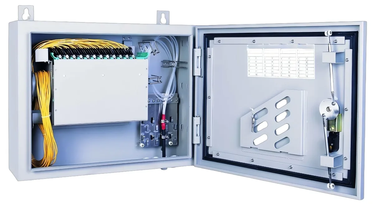
A centralised splitter at the OLT or ODF is easy to power, cool, test and secure. It also means one fibre core per subscriber from the headend to the building, which is expensive on a long or dense route. A distributed design puts a 1:8 at a street cabinet and a 1:4 or 1:8 in the building, which saves fibre but adds a second splitter, more connectors and a street cabinet to maintain. The losses add, and the second stage is often less accessible.
The field rule is accessibility. A splitter buried in a sealed ceiling box or a flooded handhole is a future fault. Put it in an ODF, a rack panel or a lockable building box, label every output and leave a service loop. If the design needs a second stage, put it where a technician can reach it without removing a ceiling.
Cascade arithmetic is simple and often ignored. A 1:8 followed by a 1:8 is a 1:64 equivalent with about 21 dB plus an extra connector pair, not 20.5 dB. A 1:64 followed by a 1:64 is 1:4096, far beyond any PON port and any sensible ONU count. The OLT port also has a maximum ONU count, typically 64, so the splitter ratio and the port limit must both pass.
The ONU count is a separate limit. A 1:64 splitter can serve 64 ONUs, and a 1:32 can serve 32, but the OLT port may be rated for 64 ONUs regardless of the splitter. A two-stage splitter network cannot exceed the OLT port limit, and a 1:64 splitter on a port rated for 32 ONUs will not register the extra units. Check both numbers before ordering.
| Topology | Split | Typical loss | Fibre count | Best for | Watch-out |
|---|---|---|---|---|---|
| Centralised at OLT | 1:32 | 16.5 dB | 1 core per subscriber | Small estate, short route | Fibre count and ODF size |
| Centralised at OLT | 1:64 | 20.5 dB | 1 core per subscriber | Dense in-building ODN | Little margin on 20 km |
| Cabinet and building | 1:8 + 1:8 | About 21 dB plus connectors | 1 core per 8 subscribers | Long feeder, dense building | Two stages, street cabinet maintenance |
| Cabinet and building | 1:8 + 1:4 | About 18 dB plus connectors | 1 core per 4 subscribers | Village or campus | Port count and splitter inventory |
Cascaded splitters add loss and connector pairs. Put both stages in the budget from the start.
How many connectors and splices should the budget carry?
Count every mated pair, not every connector. A typical FTTH path has an OLT-to-ODF patch, an ODF-to-splitter patch, a splitter-to-ODF patch, a feeder-to-building-box splice or connector, a box-to-drop connector and a drop-to-ONT connector. That is easily six to ten pairs. At 0.4 dB per pair, the connector budget is 2.4–4.0 dB before the splitter is counted.
A design with ten connector pairs has spent 4 dB before the splitter, the fibre and the splices. That is often the difference between a 1:32 and a 1:16. Reduce the count by using factory-terminated assemblies, by combining patch panels, or by moving the splitter closer to the subscriber. Do not reduce the count by omitting the ODF or the test point; those are maintenance assets, not decoration.
| Element | Typical loss | How to count | Field note |
|---|---|---|---|
| Connector pair | 0.3–0.5 dB | Every mated pair in the path | Dirty connector can add 1–3 dB |
| Splice | 0.1 dB | Every fusion or mechanical splice | Field splice quality varies; test it |
| 1:32 splitter | 16.5 dB | One per path | Add uniformity for the worst port |
| 1:64 splitter | 20.5 dB | One per path | Four dB more than 1:32 |
| Fibre, 1310 nm | 0.35 dB/km | Route length including slack | Use the cable datasheet value |
| Fibre, 1550 nm | 0.2 dB/km | CATV overlay or long haul | Lower loss, same connectors |
| WDM coupler | 0.5–1.5 dB | CATV overlay only | Budget it with the CATV receiver range |
Connector and splice counts are design inputs. If they are unknown, the budget is not finished.
What should be measured at commissioning?
Measure the OLT output at the PON port, the input to the splitter, every splitter output, and the ONT input. Record the wavelength, the meter, the value and the date. The difference between the OLT output and the ONT input is the actual path loss; compare it with the design. A 2–3 dB discrepancy usually means a dirty connector, a bad splice, a wrong splitter ratio or a macrobend, not a mysterious protocol fault.
Set a pass criterion before measuring. The link passes if the measured loss is within the design value and the residual margin after the 3 dB ageing reserve is not negative. If the measurement is 2 dB worse than design, do not adjust the criterion; find the extra loss. A re-measure after cleaning is the first step, then inspect the splices and the splitter port.
Use a calibrated meter and a reference patch cord, and test at the operating wavelength. A meter calibrated at 1310 nm will read differently at 1490 or 1550 nm; the difference is small but real. For a fault, an OTDR locates the event, but it does not replace a power meter for loss. Record the values even when the link passes; the baseline is what makes the next fault findable. A yearly spot check on critical links is enough to catch a slow degradation, provided the reading is logged against the same baseline.
| Measurement point | Instrument | Expected or reference | Record |
|---|---|---|---|
| OLT PON output | Optical power meter | Datasheet transmit power | dBm per port |
| Splitter input | Optical power meter | OLT output minus feeder loss | dBm and wavelength |
| Each splitter output | Optical power meter | Per-port test data | dBm per output port |
| ONT input | ONT diagnostic or meter | Design value with 3 dB margin | dBm and date |
| CATV receiver input | Optical power meter | +2 to −18 dBm window | dBm and RF level |
| PoF ONU DC input | Multimeter under load | Above ONU minimum input | V DC and load |
Clean and inspect every connector before measuring. A dirty connector can look like a splitter fault.
What belongs in the splitter as-built?
The as-built should identify the splitter by asset ID, ratio, serial number and location, and map every input and output port to a fibre core, a subscriber or a building. Attach the per-port insertion loss test data, the route length, the splice count and the connector polish. Add photos of the enclosure and the label, and the commissioning date and tester name.
Update the record when a port changes. A splitter port that was spare at handover becomes a subscriber drop after the first expansion; if the label and the as-built are not updated, the next technician will test the wrong port. Keep the OLT inventory and the splitter map in the same revision, and give the field team the same document the office uses.
- Splitter asset ID, ratio and serial number.
- Port map: input, outputs, cascade and spare ports.
- Per-port loss and the measured ONT receive power.
- Feeder and drop route lengths, splice count and connector polish.
- OLT port, VLAN and ONT serial for each subscriber.
- Commissioning date, meter model and tester name.
Which splitter planning mistakes show up after handover?
The most common mistake is designing on the average port. The second is using the theoretical 18 dB for a 1:64 splitter instead of the typical 20.5 dB. The third is a 1:64 splitter on a 20 km span with a high connector count. The fourth is cascading two 1:64 splitters, which produces a 1:4096 ratio that no PON port can serve. The fifth is mixing SC/UPC and SC/APC without a hybrid patch cord.
The next group is documentation. A splitter with no port map, no per-port loss and no label is a future truck roll. A design that leaves no spare ports has to add a splitter for the next subscriber. A splitter that is sealed in a ceiling box cannot be cleaned or tested. A CATV overlay that forgets the WDM coupler loss can pass the PON budget and fail the RF budget. None of these shows up on a bench test; all of them show up in the first year.
A CATV overlay adds its own failure mode. The WDM coupler adds 0.5–1.5 dB, the 1550 nm receiver has a +2 to −18 dBm window, and the RF level has to stay inside the AGC range. A PON link that passes at 1310 nm may still fail the RF channel if the 1550 nm path is at the edge of the receiver window. Measure both, and record the RF level as well as the optical power.
- Average port instead of worst case.
- Theoretical split loss instead of typical insertion loss.
- 1:64 on a long span with many connectors.
- Cascaded 1:64 plus 1:64, a 1:4096 ratio.
- UPC and APC mismatch.
- No spare ports and no spare splitter.
- No per-port test data or as-built.
What is the field rule for a splitter plan that survives?
Use 1:32 for a 20 km span, 1:64 for a short in-building ODN, and keep at least 3 dB of ageing margin after the worst-case port. Count every connector and splice, use the measured per-port loss, and write the result on the as-built. If the margin is below 3 dB, drop one ratio step or move the splitter; do not design to zero and hope the first year is kind.
The splitter is the cheapest place to change a design and the most expensive place to fix a fault. A 1:16 instead of a 1:32 costs one step of split ratio and saves 3 dB; a splitter that has to be replaced after handover costs a site visit, a re-splice and a new test record. Choose the ratio from the budget, not from the subscriber count, and prove it on the worst port.
Use this on a real site
Send the endpoint count, the longest run, the mains condition and the load. We will apply this calculation to your project and return the optical/power budget with the bill of materials.